Session 8: Capturing, Analyzing, and Balancing Training Data for Imitation Learning
In this session, you will: - Capture images from the car’s camera along with their corresponding steering angles. - Analyze the dataset to identify imbalances. - Balance the dataset to ensure fair training for a self-driving car model. - Visualize the dataset before and after balancing.
Why Is This Important?
To train a self-driving car, you need a well-balanced dataset. If most of your data represents “driving straight” while lacking examples of turns, the car might perform poorly on curved roads.
This session focuses on collecting balanced data that enables the model to handle both straight and curved paths effectively.
Libraries Used
Below are the libraries used in this session and their purposes:
rclpy: ROS 2 Python client library for creating nodes and subscribing to topics.
sensor_msgs.msg.Image: Message type used to receive camera images.
std_msgs.msg.Float32: Message type used to receive steering angles.
cv_bridge: Converts ROS images to OpenCV format for saving and processing.
os: Manages file directories for saving images and datasets.
cv2 (OpenCV): Handles image saving and processing.
pandas: Reads and manipulates the dataset.
numpy: Creates histograms for data visualization.
matplotlib: Visualizes the data with plots and graphs.
Step 1: Save Images and Steering Angles
This step involves saving images from the car’s camera along with their corresponding steering angles.
import rclpy
from rclpy.node import Node
from sensor_msgs.msg import Image  # To receive camera images
from std_msgs.msg import Float32  # To receive steering angles
from cv_bridge import CvBridge  # To convert ROS images to OpenCV
import os  # For file management
import cv2  # For saving images

# Create a folder to store images
os.makedirs("data", exist_ok=True)

# Track how many images are saved
image_count = len(os.listdir("data"))

# Create a CSV file to store image paths and steering angles
with open("data.csv", "w") as f:
    f.write("image_path,steer_angle\n")

# Variable to store the current steering angle
steer_val = None

# Callback function to handle images
def camera_cb(msg):
    global steer_val, image_count

    if steer_val is None:
        return  # Wait for a steering angle before saving an image

    # Convert ROS image to OpenCV format and save it
    image_path = f"data/{image_count}.jpg"
    bridge = CvBridge()
    image = bridge.imgmsg_to_cv2(msg, desired_encoding="bgr8")
    cv2.imwrite(image_path, image)

    # Save the image path and steering angle to the CSV file
    with open("data.csv", "a") as f:
        f.write(f"{image_path},{steer_val}\n")

    print(f"Saved {image_path} with steering angle {steer_val}")
    image_count += 1
    steer_val = None  # Reset steering angle after saving

# Callback function to handle steering angles
def steer_cb(msg):
    global steer_val
    steer_val = msg.data

# Initialize the ROS node
rclpy.init()
node = Node("data_collector")

# Subscribe to the camera and steering angle topics
node.create_subscription(Image, "/stk_image", camera_cb, 10)
node.create_subscription(Float32, "/stk_steer_val", steer_cb, 10)

# Keep the node running
try:
    rclpy.spin(node)
except KeyboardInterrupt:
    print("Stopping data collection...")
finally:
    rclpy.shutdown()
Explanation:
Image Subscription: Subscribes to /stk_image to receive images from the camera.
Steering Angle Subscription: Subscribes to /stk_steer_val to get the steering angle values.
Saving Images: The images and their corresponding steering angles are saved in a data folder and recorded in a data.csv file.
Note
Do 2-3 laps in map forward direction and 2-3 laps in reverse direction to collect a diverse dataset. This avoids overfitting to a specific driving style.
Step 2: Analyze the Dataset
Once the data is collected, it’s time to analyze the distribution of steering angles to check for imbalance. For example, if the dataset has too many “straight-driving” examples, the car may struggle with turns.
Note
Ensure you have the data.csv file saved with image paths and steering angles before proceeding. It should be in the same directory as the script.
Note
From here we will use Jupyter Notebook for data analysis and visualization. The code snippets can be run in a Jupyter Notebook environment. The file extension for Jupyter Notebook is .ipynb.
import pandas as pd  # For data analysis
import matplotlib.pyplot as plt  # For data visualization
import numpy as np  # For numerical operations

# Load the dataset
data = pd.read_csv("data.csv")
data = data.dropna(subset=["steer_angle"])

# Plot a histogram of the steering angles
num_bins = 25
hist, bins = np.histogram(data["steer_angle"], num_bins)
center = (bins[:-1] + bins[1:]) / 2

plt.bar(center, hist, width=0.05)
plt.xticks([-1, 0, 1], ['Right', 'Center', 'Left'])
plt.gca().invert_xaxis()  # Reverse the x-axis
plt.xlabel("Steering Angle")
plt.ylabel("Frequency")
plt.title("Distribution of Steering Angles")
plt.show()
Explanation:
pandas: Loads the data.csv file and organizes the data.
numpy: Computes the histogram to group steering angles into bins.
matplotlib: Visualizes the histogram to show how many examples are in each bin.
Following figure shows the distribution of steering angles in the dataset:
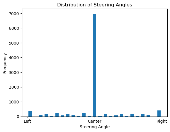
From the histogram, you can see how many examples are available for each steering angle, showing a lot of straight-driving examples and fewer turning examples.
Step 3: Balance the Dataset
To prevent bias toward straight driving, we’ll balance the dataset by reducing the number of straight-driving examples.
# Separate straight-driving and turning examples
straight_data = data[data["steer_angle"] == 0]
turning_data = data[data["steer_angle"] != 0]

# Randomly sample fewer straight-driving examples
straight_data = straight_data.sample(len(turning_data) // 2)

# Combine straight and turning examples into a balanced dataset
balanced_data = pd.concat([straight_data, turning_data])

# Save the balanced dataset
balanced_data.to_csv("balanced_data.csv", index=False)

print(f"Original dataset size: {len(data)}")
print(f"Balanced dataset size: {len(balanced_data)}")
Explanation:
Why Balance?: If the dataset is imbalanced, the car will overfit to driving straight and fail on turns.
Random Sampling: Keeps only a limited number of straight-driving examples to match the number of turning examples.
Step 4: Visualize the Balanced Dataset
After balancing, visualize the new dataset to confirm the improvement.
# Plot the histogram of the balanced dataset
hist, bins = np.histogram(balanced_data["steer_angle"], num_bins)
center = (bins[:-1] + bins[1:]) / 2

plt.bar(center, hist, width=0.05)
plt.xticks([-1, 0, 1], ['Right', 'Center', 'Left'])
plt.gca().invert_xaxis()  # Reverse the x-axis
plt.xlabel("Steering Angle")
plt.ylabel("Frequency")
plt.title("Balanced Distribution of Steering Angles")
plt.show()
Following figure shows the balanced dataset after reducing the number of straight-driving examples:
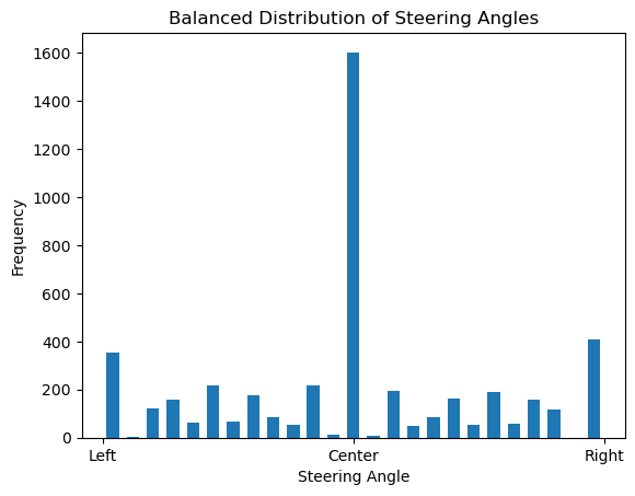
The balanced dataset now has an equal number of straight-driving and turning examples, ensuring fair training for the self-driving car.
Summary
In this session, you:
Collected images and steering angles using ROS 2 and OpenCV.
Analyzed the dataset for imbalances.
Balanced the dataset to ensure fair training.
Visualized the data before and after balancing.
This process ensures that your self-driving car learns to handle both straight roads and turns effectively. In the next session, we’ll train a neural network using this balanced dataset. Stay tuned!